Fraud in Modern Finance – Part 4: Misuse of Statistics and Other Controversial Practices | dance with the trend

Note to readers: This is the fourth time. series of articles I am publishing here an excerpt from my book “Investing in Trends”. I hope you found this helpful. Market myths are usually perpetuated by repetition, misleading symbolic connections, and complete ignorance of the facts. The world of finance is full of these trends. Let’s look at some examples here. Keep in mind that while not all of these examples are completely misleading and sometimes even valid, there are too many loopholes to make them worthwhile as an investment concept. And not everything is directly related to investing and finance. enjoy! – Greg
average deception
The world of finance is full of misinformation.
In particular, the use of averages is a matter that requires discussion. Figure 4.1 shows compound returns for different asset classes. If I were selling you a buy and hold strategy or index funds, you would love this chart. Looking at the 85 years of data shown here, we can say that if you invested in small-cap stocks, the average annual return was 11.95%, and if you invested in large-cap stocks, you could say that the average annual return was 9.85%. Percent per year. And I will be correct.
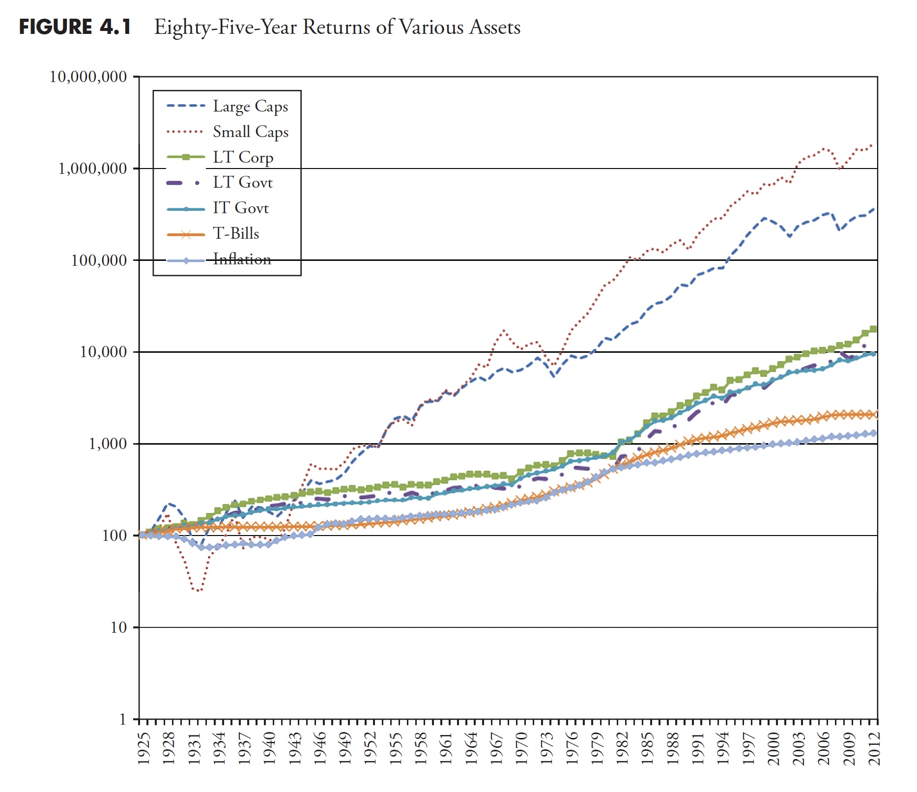 Figure 4.1
I think most investors have about 20, maybe 25 years to accumulate retirement assets. People in their 20s and 30s find it difficult to save a lot of money for a variety of reasons, including low income, children, materialism, and college. So, based on that information, what’s wrong with this chart? It means investing for 85 years, but a person cannot invest for 85 years. As we said earlier, it takes most people about 20 years to build up their retirement assets. And there are many 20-year periods in this chart where returns were terrible. The bear market that began in 1929 did not fully recover until 25 years later in 1954. 1966 took 16 years to recover, 1973 took 10 years, and as of 2012, the 2000 bear still has not recovered.
Table 4.1 shows performance figures for the asset classes shown in Figure 4.1 (LT – Long Term, IT – Medium Term). The cumulative numbers in Table 4.1 start at 1 on December 31, 1925.
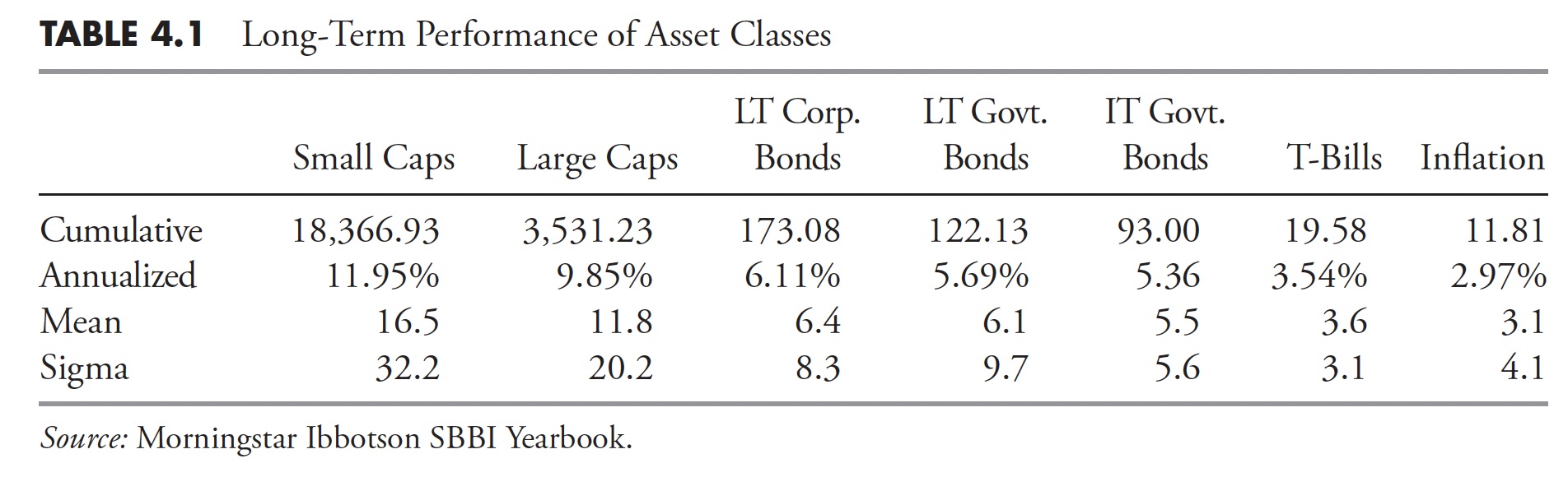 Table 4.1Hint: If someone uses inappropriate averages, be careful. Or, more accurately, inappropriate use of averages.
Recall from Table 4.1 that the compound returns for small and large stocks were approximately 12% and 10%, respectively. Figure 4.2 shows 10-year rolling returns by range since 1900. Rolling returns mean they represent periods such as 1900-1909, 1901-1910, 1902-1911, etc. It is clear that the small- and large-cap returns depicted in Table 4.1 fall in the mid-range (8 to 12%) of Figure 4.2, but only 22% of the entire 10-year rolling period falls in the mid-range. That range. Often the average is not that average. It reminds me of the story of the 6-foot-tall Texan who drowned while crossing a stream whose average depth was only 3 feet.
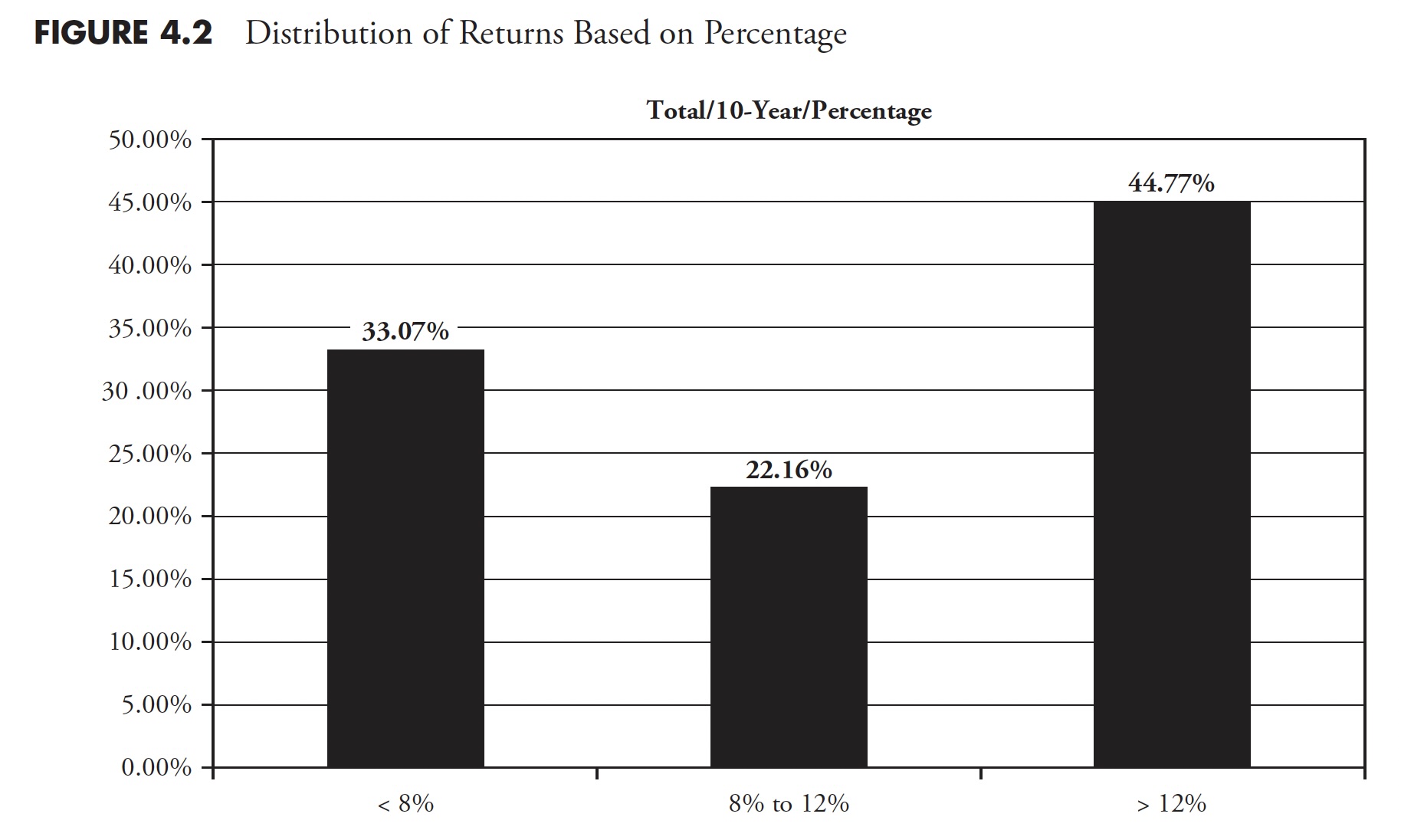 Figure 4.2
Another (and final) example shows how easy it is to get confused about what an average is. Of course, this time it was intentional. This example should put this into perspective. Rates of change cannot be linearly related. In Figure 4.3, point A is 20 miles from point B. If you drive 60 mph from point A to point B and back from point B to point A, you are driving 30 mph. What was his average speed while you were on the road?
A. 55 miles per hour
B. 50 miles per hour
C. 45 miles per hour
D. 40 miles per hour
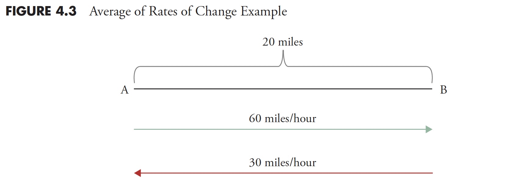 Figure 4.3
Many people will answer 45 mph ((60 mph + 30 mph)/2). However, rates of change cannot be averaged out like constants and linear relationships. Distance is speed multiplied by time (d = RT). So time (tea) is the distance (d)/ratio (R). The first leg, from A to B, is 20 miles divided by 60 mph, or 1/3 of an hour. The second leg, from B to A, is 20 miles divided by 30 mph, or 2/3 of an hour. Adding it twice (1/3+2/3 = 1 hour) gives you a 1-hour trip, a total distance of 40 miles, and an average speed of 40 mph. If you want more information about this, look up the harmonic mean. This is because it is the correct way to determine the central tendency of data when it is in the form of a ratio or ratio.
Figure 4.4 shows 20 years of rolling price returns for the Dow Industrials. Returns for this 127-year sample (1885-2012) range from a low of 0.3.71% on August 31, 1949 to a high of 14.06% on March 31, 2000, or 17.77%. .
To clarify rolling returns, if investors were in the Dow Industrials from September 30, 1929 to August 31, 1949 (the aforementioned low point), the return was 0.3.71%. Complementarily, if they had invested on April 30, 1980, on March 31, 2000 they would have earned a return of 14.06%. The average return is 5.2% and the median return is 4.8%. If the median is less than the average, it simply means that more returns were below the average. If we recall the often used long-run assumption from the first part of this chapter (Figure 4.1), we can see that it is problematic. The magnitude of the error in long-term return assumptions cannot be overstated or ignored. This volatility in returns can mean a completely different retirement environment for investors who use these long-term assumptions about future returns. It could be the difference between living like a king and living on government support. The same problem arises when institutional investors use these long-term averages.
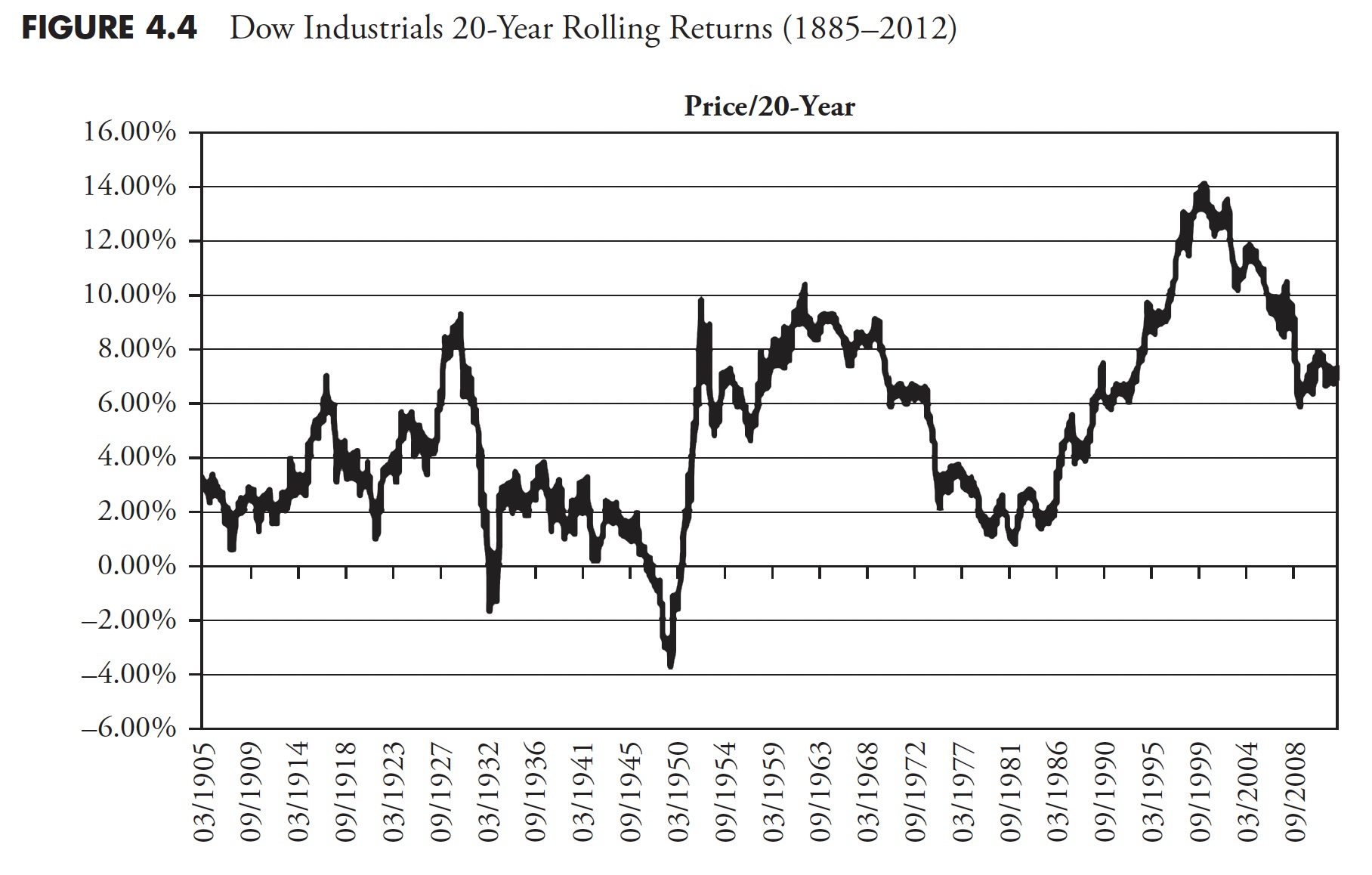 Figure 4.4
As the architect of modern portfolio theory, one of the key beliefs developed by Markowitz in the 1950s was the specification of inputs for an efficient investment portfolio. In fact, his focus wasn’t on input at all. The inputs required are expected future returns, volatility and correlation. The industry as a whole has taken an easy approach to solving this problem by leveraging long-term averages for inputs. This means that you take a full swing through all the available data at once, and the average is what is used for input. Otherwise, it’s a pretty good theory. These long-term investments are completely inappropriate for most investors’ investment horizons. In fact, I think it is inappropriate for all humans. Delving deeper into this is not the topic of this book, but it once again brings to light the terrible misuse of averages. These inputs should use averages appropriate to the investor’s accumulation period.
One by land, two by sea
Sam Savage is Professor of Management Science and Engineering Consulting at Stanford University and a Fellow of the Judge Business School at the University of Cambridge. He wrote an insightful book. flaw in the averageIn 2009, he included a short story called “The Red Coats” that fits perfectly into this chapter.
Spring 1775: Colonists are concerned about British plans to raid Lexington and Concord, Massachusetts. The Boston Patriots develop a plan that explicitly considers a variety of uncertainties. The British army would come by land or sea. These unknown pioneers of modern decision analysis did the right thing by explicitly planning for two situations. If Paul Revere and the Minutemen had planned a single average scenario where the British would walk on the beach with one foot on land and the other in the sea, North American citizens today may speak with different accents.
Incidentally, Dr. Savage’s father, Leonard J. Savage, wrote the seminar. basics of statistics He was a renowned mathematical statistician who worked closely with Milton Friedman in 1972.
Everything with four legs is a pig
Although it has nothing to do with investing or finance, it is a story about averages that provides additional support to this topic. Doctors use growth charts (height and weight charts) as a guide to a child’s growth. What people don’t realize is that it was created by actuaries for insurance companies, not doctors. As doctors began to use this term, it became Overweight, underweight, obesity, etc. are based on averages. So if your doctor tells you that you are overweight and need to lose weight, he or she is also telling you that you need to lose weight to become average. and wall street journal July 24, 2012 article by Melinda Beck, “The broad changes are due in part to rising obesity rates, more premature babies surviving, and an increasingly diverse population. But the Centers for Disease Control and Prevention’s official growth charts show that the CDC and “The prevention still reflects the size distribution of American children in the 1960s, 1970s, and 1980s. The CDC has said it has no plans to adjust the charts because it does not want more and more obese people to reach a new standard.” And now you know.
At my last physical, I told my doctor that this chart of height and weight was just a big average created by the insurance company’s actuaries and that it was okay to be above average. The next chapter focuses on the multi-billion dollar forecasting industry. I am rarely invited to appear in the financial media anymore because I refuse to make predictions. It’s a fool’s game.
Thank you for reading this far. I plan to publish one article in this series each week. Can’t wait? The book is on sale here.


