View more uncle statistics | Ethereum Foundation Blog

Here are some interesting results on the performance of various miners during the first 280,000 blocks of the Ethereum blockchain. During this time I collected a list of blocks and uncle Coinbase addresses. You can find the raw data here is a block and here for my uncleAnd this allows us to gather a lot of interesting information, especially about stale fees and how well connected various miners and pools are.
First, here is the scatterplot:
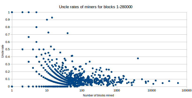
What we can clearly see here are a few key trends. First of all, the uncle rate is significantly lower than in the Olympics. In total, we saw 20,750 uncles with 280,000 blocks, or an uncle rate of 7.41% (if we calculate this comprehensively, i.e. count uncles as a percentage of all blocks rather than uncles per block, we get 6.89%). Much higher than similar figures Bitcoin in 2011, the mining ecosystem was more similar to Ethereum in that CPUs and GPUs were still dominant and transaction volumes were low. This does not mean that miners only get 93.11% of what they would earn if they were infinitely well connected to everyone else. Ethereum’s uncle mechanic effectively eliminates ~87% of the difference, so the actual “average loss” due to poor connectivity is only ~0.9%. This means that as more transactions begin to occur on the network, these losses will increase for two reasons. First, the uncle mechanic only works with basic block rewards, not transaction fees, and second, the larger the block, the longer the propagation time is bound to be.
Second, we can see that there is a general trend for large miners to have lower uncle rates. Of course, this is to be expected, but to what extent is it difficult to analyze (1) why this happens, (2) if this is actually a real effect, and not simply a statistical artifact of the fact that smaller samples tend to occur? This is important. This will lead to more extreme results.
Breaking down by miner size, the statistics are as follows:
| Number of blocks mined | Average Uncle Ratio |
| <= 10 | 0.127 |
| 10-100 | 0.097 |
| 100-1000 | 0.087 |
| 1000-10000 | 0.089* |
| >= 10000 | 0.055 |
* These results may have been significantly skewed by a single outlier, i.e. a miner who is likely a broken miner (0.378 uncle ratio), a dot on the chart at block 4005 mined. Not including these miners, the average uncle ratio is: 0.071 This seems much more in line with the general trend.
There are four basic hypotheses that could explain these results.
- expertise gap: Large miners have professional operations and have more resources to invest in improving the overall connectivity to the network (e.g. buying better wireless, making sure uncle rates are sub-optimal due to networking issues) by observing more carefully). It has higher efficiency. Small-scale miners, on the other hand, tend to use laptops as a hobby and may not have particularly good internet connections.
- last block effect: The miner who created the last block waits ~1 second for the block to propagate through the network and then immediately “learns” about the block, thus gaining an advantage in finding the next block.
- pool efficiency: Very large miners are pools, and pools are likely to be associated with more efficient networking than solo miners for some reason.
- period difference: In the first days of the blockchain, when block times were very fast and uncle rates were very high, pools and other large-scale miners were inactive.
The final block effect doesn’t clearly tell the whole story. If the cause is 100%, you will actually see a linear decrease in efficiency. A miner who mined 1 block would see an uncle rate of 8%, while a miner who mined 28000 blocks (i.e. 10% of the total) would see an uncle rate of 7.2%. Uncle ratio (%), miners who mined 56000 blocks will see a 6.4% uncle ratio, etc. This is because a miner who has mined 20% of the blocks has been mining the latest block for 20% of the time, thus reducing the benefit of the 0% expected uncle rate by 20%, from 8% to 6.4% for 20%. The difference between a miner who mined 1 block and a miner who mined 100 blocks is negligible. Of course, in reality, the decline in default rates as size increases appears to be almost perfectly logarithmic. This curve seems much more consistent with expertise gap theory than any other. The lag theory is also supported by the curve, but it is important to note that only ~1600 uncles (i.e. 8% of all uncles and 0.6% of all blocks) were mined during the first two busy days when the uncle rate was high. So that could account for ~0.6% of the maximum uncle rate.
The fact that the expertise gap appears to be dominant is in some ways an encouraging sign. Particularly because (i) this factor is more important at small and medium scales than at medium and large scales and (ii) individual miners tend to be economically offset. A bigger factor than the loss of efficiency is the fact that you’re using hardware that you’ve already largely paid for.
Now how about jumping from 7.1% for 1000-10000 blocks to 5.5% for everyone above that? The last block effect can explain about 40% of the effect, but not all. 9% should be expected to decrease from 7.1* to 7.1% * 0.93 = 6.4%, but it is important to note that given the small number of miners, the findings here should be taken as very tentative at best.
The main characteristics of miners over 10000 blocks are of course: them is swimming pool (or at least 3 out of 5; different two They are the smallest miners, but they are solo miners.) Interestingly, the uncle rates for the two non-pools are 8.1% and 3.5% respectively, which is a weighted average of 6.0%, which is not very different from the weighted average old rate of 5.4% for the three pools. So, in general, pools seem to be slightly more efficient than solo miners, but again, that result should not be considered statistically significant. Although the sample size within each pool is very large, the sample size of the pools is small. Moreover, the more efficient mining pool is not actually the largest mining pool (nanopool), but Sprnova.
This raises an interesting question for us. Where do the efficiency and inefficiency of joint mining come from? On the one hand, the pool is very well connected to the network and does a good job of distributing its own blocks. They also benefit from a weaker version of the last block effect (weaker version because there is still a single hop round trip from miner to pool to miner). On the other hand, any delay in fetching work from the pool after creating a block slightly increases the stale rate. That is, assuming a network latency of 200ms, it’s around 1%. These forces are likely to roughly cancel out.
The third key thing to measure is how much of the gap we see is due to true inequality in how well connected the miners are, and how much is due to random chance. To check this, we can perform a simple statistical test. Below are the uncle rate deciles for all miners who produced 100 or more blocks (e.g. the first number is the lowest uncle rate, the second number is the 10th percentile, the third number is the 20th percentile, etc., and the last number is continues until). highest):
(0.01125703564727955, 0.03481012658227848, 0.04812518452908179, 0.0582010582010582, 0.06701030927835051, 0.07642487046632124, 0.0847457627118644, 0.09588299024918744, 0.11538461538461539, 0.14803625377643503, 0.3787765293383271)
Below are deciles generated by a random model where the “natural” default rate for all miners is 7.41% and all gaps are due to some luck or unluckiness.
(0.03, 0.052980132450331126, 0.06140350877192982, 0.06594885598923284, 0.06948640483383686, 0.07207207207207207, 0.07488986784140969, 0.078125, 0.08302752293577982, 0.09230769230769231, 0.12857142857142856)
So we get roughly half the effect. The other half actually comes from true connectivity differences. In particular, if we do a simple model where the “natural” stale rate is a random variable normally distributed around a mean of 0.09, a standard deviation of 0.06, and an absolute minimum of 0, we get:
(0, 0.025374105400130124, 0.05084745762711865, 0.06557377049180328, 0.07669616519174041, 0.09032875837855091, 0.10062893081761007, 0.11311861743912019, 0.13307984790874525, 0.16252390057361377, 0.21085858585858586)
It grows too fast on the low end and slow on the high end, but this is pretty close. In reality, there appears to be a “natural failure rate distribution” that works best. positive skewness, we expect to see diminishing returns from the increasing effort put into making networks increasingly better connected. In general, the effect is not very significant. If you divide by 8, especially after taking into account the uncle mechanism, the gap is much smaller than the gap in electricity costs. Therefore, the best approach to improve decentralization in the future is very focused on creating more decentralized alternatives to mining pools. Perhaps a mining pool that implements something like Meni Rosenfeld. Multiple PPS This could be a medium-term solution.


